OpenTURNS#
Test.
import micropip
await micropip.install("openturns", keep_going=True)
# this cell is just to make testing easier, since the one above has remove input tag
# import micropip
# await micropip.install("openturns", keep_going=True)


# %pip install package_name
import openturns as ot
import openturns.viewer as viewer
from matplotlib import pylab as plt
ot.Log.Show(ot.Log.NONE)
import numpy as np

x = ot.Normal(4).getSample(6)
print('OpenTurns Sample:\n\n', x)

y = np.array(x)
print('\nOpenTurns Sample converted to numpy array:\n\n', y)
OpenTurns Sample:

     [ X0         X1         X2         X3         ]
0 : [  0.608202  -1.26617   -0.438266   1.20548   ]
1 : [ -2.18139    0.350042  -0.355007   1.43725   ]
2 : [  0.810668   0.793156  -0.470526   0.261018  ]
3 : [ -2.29006   -1.28289   -1.31178   -0.0907838 ]
4 : [  0.995793  -0.139453  -0.560206   0.44549   ]
5 : [  0.322925   0.445785  -1.03808   -0.856712  ]

OpenTurns Sample converted to numpy array:

 [[ 0.60820165 -1.2661731  -0.43826562  1.2054782 ]
 [-2.18138523  0.35004209 -0.35500705  1.43724931]
 [ 0.81066798  0.79315601 -0.4705256   0.26101794]
 [-2.29006198 -1.28288529 -1.31178112 -0.09078383]
 [ 0.99579323 -0.13945282 -0.5602056   0.4454897 ]
 [ 0.32292503  0.4457853  -1.03807659 -0.85671228]]
sample = ot.Normal(4).getSample(6)
print('OpenTurns Sample:\n\n', sample)
OpenTurns Sample:

     [ X0         X1         X2         X3         ]
0 : [  0.473617  -0.125498   0.351418   1.78236   ]
1 : [  0.0702074 -0.781366  -0.721533  -0.241223  ]
2 : [ -1.78796    0.40136    1.36783    1.00434   ]
3 : [  0.741548  -0.0436123  0.539345   0.29995   ]
4 : [  0.407717  -0.485112  -0.382992  -0.752817  ]
5 : [  0.257926   1.96876   -0.671291   1.85579   ]
It’s possible to get one value from a point
print('The second point in the above point is: {0:.3f}'.format(sample[1][1]))
The second point in the above point is: -0.781
Thus it’s also possible to export a point as a list since Samples and Points have list comprehension.
pythonlist = [value for value in sample[1]]
print(f'The second Point has values: ',*[f'{pythonlist:.3f}' for pythonlist in pythonlist])
print('but now it has type ',type(pythonlist))
The second Point has values:  0.070 -0.781 -0.722 -0.241
but now it has type  <class 'list'>
It’s harder to access all points for one of the dimensions from a sample, but fortunately, a Sample has a method asPoint() which gives the values of a 1D sample as a point!
sampleaspoint = sample[:,0].asPoint()
print('\nValues for the first variable are: ',*[f'{i:.3f}' for i in sampleaspoint])
print('with type ',type(sampleaspoint))
Values for the first variable are:  0.474 0.070 -1.788 0.742 0.408 0.258
with type  <class 'openturns.typ.Point'>
Example: reliability of a simple slope#
This is from Baecher and Christian (2003), also used in Moss (2020).
Simple wedge failure with self-weight balanced by cohesion \(c\). Clacluate load as \(S=0.25\gamma H\), where \(h=10\) m. Distributions are normal, where \(\gamma\sim\)N(\(\mu_\gamma=20\) kPa, \(\sigma_\gamma=2\) kPa) and \(c\sim\)N(\(\mu_c=100\) kPa, \(\sigma_c=30\) kPa).
\(Z=R-S=c-0.25\gamma H\)
Results: \(\beta=1.64\) and \(p_f=0.051\).
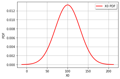
Start by defining the random variables and plotting the distributions.
cohesion = ot.Normal(100,30)
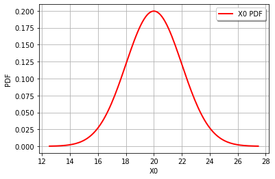
gravity = ot.Normal(20,2)
height = 10
graph = cohesion.drawPDF()
view = viewer.View(graph)
graph = gravity.drawPDF()
view = viewer.View(graph)
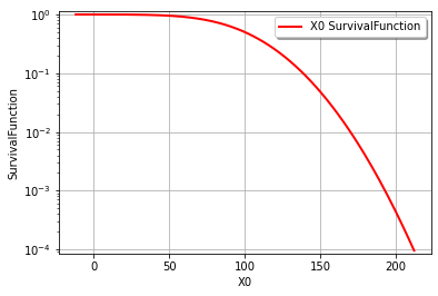
It’s also easy to draw the CDF or inverse CDF and make a logarithmic axis. This page is a good starting point for formatting hints.
graph = cohesion.drawSurvivalFunction()
graph.setLogScale(ot.GraphImplementation.LOGY)
view = viewer.View(graph)
It’s actually very easy to combine distributions in OT. The distribution for a function of random variables (i.e., theoretically and as an OT distribution class) can be evaluated as if they were normal Python variables for addition, multiplication and division using the distributions or scalar values. Thus, for our example, we can combine the distributions for \(R\) and \(S\) directly and solve for the reliability index exactly with just 2 lines. Note: this isn’t just limited to normal distributions, OT can do a lot. See quick start and distribution manipulation example pages. See the transformation page for a list of functions that can be used to transform distributions (e.g., you can’t use \(x^2\), but must use sqr(x)). These functions are methods in the distribution class.
Z = cohesion - 0.25*gravity*height
print('Z becomes a distribution class: ',type(Z),'\n')
beta = Z.getMean()[0]/Z.getStandardDeviation()[0]
pf = Z.computeCDF(0)
print('The reliability index is ',beta)
print('The failure probability is ',pf,'\n')
print('The original distribution for c = ',cohesion)
print('The original distribution for g = ',gravity,'\n')
print('The combined distribution for Z = ',Z)
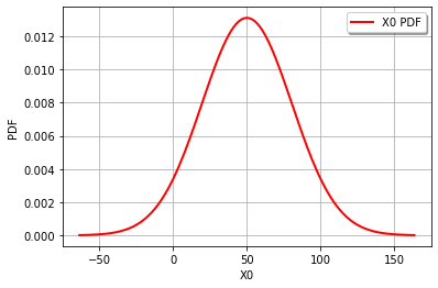
graph = Z.drawPDF()
view = viewer.View(graph)
Z becomes a distribution class:  <class 'openturns.model_copula.Distribution'>

The reliability index is  1.643989873053573
The failure probability is  0.050089147113134

The original distribution for c =  Normal(mu = 100, sigma = 30)
The original distribution for g =  Normal(mu = 20, sigma = 2)

The combined distribution for Z =  Normal(mu = 50, sigma = 30.4138)
Z = cohesion - 0.25*gravity*height
print(cohesion, gravity, Z)
Normal(mu = 100, sigma = 30) Normal(mu = 20, sigma = 2) Normal(mu = 50, sigma = 30.4138)
Example: reliability of a thingamajig#
This is from the April 2021 exam for CIE4130 Probababilistic Design, which is looking at the design of a thingamajig. The limit-state function is \(Z=y-x^{0.5}-2\) where \(x\sim\)N\((\mu_x=4.0,\sigma_x=0.5)\) and \(y\sim\)N\((\mu_y=5.0,\sigma_y=0.5)\)
x = ot.Normal(4.0,0.5)
y = ot.Normal(5.0,0.5)
Z = y - x.sqrt() - 2
print('Z becomes a distribution class: ', type(Z), '\n')
beta = Z.getMean()[0]/Z.getStandardDeviation()[0]
pf = Z.computeCDF(0)
pfN = ot.Normal(0,1).computeCDF(-beta)
print('The reliability index is ', beta)
print('The failure probability is ', pf, ', using P[Z<0], whereas')
print('the failure probability is ', pfN, ', using Phi[-beta]\n')
print('The original distribution for x = ', x)
print('The original distribution for y = ', y, '\n')
print('The combined distribution for Z = ', Z)
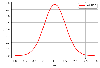
graph = Z.drawPDF()
view = viewer.View(graph)
Z becomes a distribution class:  <class 'openturns.model_copula.Distribution'>

The reliability index is  1.947161998215974
The failure probability is  0.025680273921256845 , using P[Z<0], whereas
the failure probability is  0.025757658031434517 , using Phi[-beta]

The original distribution for x =  Normal(mu = 4, sigma = 0.5)
The original distribution for y =  Normal(mu = 5, sigma = 0.5)

The combined distribution for Z =  RandomMixture(-CompositeDistribution=f(Normal(mu = 4, sigma = 0.5)) with f=[x]->[sqrt(x)] + Normal(mu = 3, sigma = 0.5))
Setting up a function and random vectors#
A random vector is how a random variable is represented. Each variable has an underlying distribution (or several marginals and a defendence structure). A CompositeRandomVector is a function of random variables and is easily defined with the function and RandomVector as inputs. There are several options for specifying a function. See the quick-start guide and other short exmaples described here.
Overview functions#
PythonFunction is a class in OT which is defined as follows”
PythonFunction(nbInputs, nbOutputs, myPythonFunc)
where
nbInputs: the number of inputs,nbOutputs: the number of outputs,myPythonFunc: a Python function.
Input and outputs are ‘vectors’ (i.e., 1D objects), but inputs are restricted to the OT Point class: y = myPythonFunc(x), thus
def myPythonFunc(x):
    [...]
    return y
Vectorizing the function allows all the points in a sample to be evaluated without making a for loop, but requires conversion to a numpy array. Note: it’s possible to convert all points for each random variable to lists, but I’m not sure if this is more computationally efficient than converting to a numpy array.
import numpy as np

def myPythonFunc(x):
    x = np.array(x)
    x0 = x[:, 0]
    x1 = x[:, 1]

    y0 = mysubfunction1(x0, x1)
    y1 = mysubfunction2(x0, x1)

    y = np.vstack(y0, y1)

    return y
To call a vectorized function, the following func_sample option must be set:
myfunction = PythonFunction(nbInputs, nbOutputs, func_sample = mySimulator)
Symbolic functions can be used to speed up performance and allow derivatives to be computed exactly. The function is defined as follows, with inputs and formulas given as a list of strings:
myfunction = SymbolicFunction(list_of_inputs, list_of_formulas)
Python function and vectorized Python function example#
First a Python function. A few notes to remember:
vectorize input, vector out
can speed up calculations by allowing the function to take a Sample
Samples can only handle addition and multiplication, otherwise need numpy (thus only vectorize if calculation is worth the overhead of numpy array conversion; see
myLSF2)for vectorized functions, use the following option to enable evaluation with a sample, as opposed to a point:
func_sample = myfun
Running the two functions below took longer for the vectorized one. Probably because the vector needed to be converted to array and saved.
import time
import numpy as np

# define marginals
x = ot.Normal(4.0, 0.5)
y = ot.Normal(5.0, 0.5)

# multivariate distribution (with independent marginals)
inputDistribution = ot.ComposedDistribution((x, y))
# random vector for generating realizations
inputRandomVector = ot.RandomVector(inputDistribution)

# define the limit-state function
def myLSF(x):
    Z = x[1] - x[0]**0.5 - 2
    y = [Z]
    return y

# create the function of random variables
myfunction = ot.PythonFunction(2, 1, myLSF)
outputvector = ot.CompositeRandomVector(myfunction, inputRandomVector)

# sample
montecarlosize = 10000
t1 = time.time()
outputSample = outputvector.getSample(montecarlosize)
t2 = time.time()

print('Sample mean = ', outputSample.computeMean()[0])
print('Sample stdv = ', outputSample.computeStandardDeviation()[0, 0])
print('calculation took ', t2-t1, ' seconds')

# now create a vectorized function, which requires numpy arrays
def myLSF2(x):
    x = np.array(x)
    Z = x[:, 1] - x[:, 0]**0.5 - 2
    y = np.vstack(Z)
    return y

# create the vectorized Python function using the func_sample option
myfunctionVect = ot.PythonFunction(2, 1, func_sample = myLSF2)
#it is easy to enable the history, but expensive for computation time
#myfunction = ot.MemoizeFunction(myfunction)
outputvector2 = ot.CompositeRandomVector(myfunctionVect, inputRandomVector)

#sample
t1 = time.time()
outputSample2 = outputvector2.getSample(montecarlosize)
t2 = time.time()

print('Sample mean = ', outputSample2.computeMean()[0])
print('Sample stdv = ', outputSample2.computeStandardDeviation()[0, 0])
print('calculation took ', t2 - t1, ' seconds')
# note the way std dev was accessed - as a matrix!
Sample mean =  1.0144595929476583
Sample stdv =  0.524804927305712
calculation took  0.059850454330444336  seconds
Sample mean =  1.0124297386094485
Sample stdv =  0.5211331101231553
calculation took  0.03390836715698242  seconds